Correlation means two variables change together; causation means a change in one produces a change in the other. A correlation sometimes comes from a cause, but it also arises from chance, from the effect running the other way, from a third variable, or from the way the sample was chosen. This guide to correlation vs causation shows all four, a worked example you can recompute, and how to word each kind of finding in a paper.
Key Takeaways
- A correlation coefficient, r, runs from −1 to +1 and describes how closely two variables move together. It says nothing about which one, if either, drives the other.
- Four things produce a correlation when X does not cause Y: chance, reverse causation, a third variable (confounding) and the way the sample was selected (collider bias).
- In our 10-child example, shoe size and reading score correlate at r = 0.93. Holding age constant, the correlation is exactly 0.
- “Correlation does not imply causation” does not mean a correlation rules causation out. In one Introductory Psychology exam, 31% of 124 students made that mistake, answering that causation was impossible in either direction.
- Researchers build a causal case with randomized experiments, natural experiments and Bradford Hill’s nine viewpoints. In a paper, write “associated with” for a correlational result and keep “caused” for evidence that supports it.
What is the difference between correlation and causation?
Correlation is a statistical pattern: as one variable rises, the other tends to rise (a positive correlation) or fall (a negative one). Causation is a claim about intervening: change one variable and the other changes because of it. The Australian Bureau of Statistics (ABS) puts the gap plainly: a correlation “does not automatically mean that the change in one variable is the cause of the change in the values of the other variable.”
| Correlation | Causation | |
|---|---|---|
| What it says | X and Y vary together | Changing X changes Y |
| How it is measured | A coefficient such as Pearson’s r, from −1 to +1 | An effect estimate from a design that rules out other explanations |
| Typical design | Observational: surveys, records | A randomized experiment, or several kinds of evidence judged together |
| Direction | Symmetric: r for X and Y equals r for Y and X | One way: X → Y |
| Wording in a paper | “X was associated with Y” | “X increased Y” |
| Example | Shoe size and reading score in children | Smoking and lung cancer |
Penn State’s STAT 200 notes put the rule in one line, “Correlation does NOT equal causation”, and add that a strong relationship between x and y could mean y causes x, or that a confounding variable causes both. Their rough scale for the size of r: 0 to 0.2 very weak, 0.2 to 0.4 weak, 0.4 to 0.6 moderate, 0.6 to 0.8 strong, 0.8 to 1.0 very strong.
Strength settles nothing in either direction. A very strong r is entirely non-causal in the worked example below. And because r measures straight-line relationships, the ABS notes that a real relationship that is not a straight line can give a coefficient closer to 0.
Why doesn’t correlation imply causation?
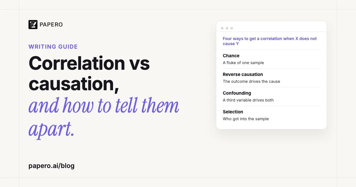
Because at least four other processes produce the same pattern. The correlation is a fluke of one sample (chance). The outcome drives the supposed cause (reverse causation). A third variable drives both (confounding). Or the way people got into the sample ties the two together (selection or collider bias). A causal claim has to rule out all four, including the ones that do not come to mind first.
| Explanation | What happens | Example | How researchers check |
|---|---|---|---|
| Chance | The pattern appears in one sample by luck | With 10 pairs of unrelated numbers, about 1 sample in 20 gives r of 0.63 or more in either direction | Larger samples, replication, a hypothesis stated in advance |
| Reverse causation | Y changes X | Early stages of a disease change a person’s diet | Measure the supposed cause before the outcome |
| Confounding | A third variable drives X and Y | Warm weather raises both ice cream sales and crime | Measure it and adjust, or randomize |
| Selection (collider) bias | X and Y both affect who ends up in the sample | Academic and sporting ability at a selective school | Sample the whole population; ask who is missing |
Chance
Small samples produce large correlations by luck. With 10 pairs, r has to reach 0.632 (in either direction) to pass a two-tailed test at the 0.05 level; we drew 100,000 samples of 10 pairs of unrelated random numbers, and 5.1% crossed that line. Test 20 unrelated pairs independently and the chance that at least one comes out “significant” is 1 − 0.9520, about 64%.
The medical statistician Austin Bradford Hill gave tests of statistical significance a modest job in a 1965 paper: they “can, and should, remind us of the effects that the play of chance can create”, and beyond that, he wrote, they contribute nothing to the proof of a hypothesis.
Reverse causation
Hill called this temporality: “which is the cart and which the horse?” His example: “Does a particular diet lead to disease or do the early stages of the disease lead to those peculiar dietetic habits?” A survey that measures both variables at once cannot tell which came first, the main limit of a cross-sectional study. Measuring the supposed cause before the outcome removes this explanation, though not the other three.
Confounding
OpenStax’s Psychology 2e uses ice cream consumption and crime: both rise when temperatures are warmer, so temperature is “a confounding variable that could account for the relationship between the two variables.” Our guide to confounding variables and how to control them covers the five standard controls, from random assignment to regression.
Selection and collider bias
Griffith and colleagues define a collider as “a variable that is influenced by two other variables”, for example when a risk factor and an outcome both make a person more likely to be sampled. Their illustration will be familiar to students: if academic and sporting ability each help a student get into a prestigious school, the two traits are “negligibly correlated in the general population” but strongly correlated among the students admitted.
A survey of one honours programme or one online forum can have the same problem, and so can a sample of volunteers, whenever both variables affect who joins (see our guide to convenience sampling). Adjusting for a collider adds bias instead of removing it: colliders become an issue, Griffith and colleagues write, “when they are conditioned upon in analysis”.
A worked example: shoe size, reading and age
Here are invented data for 10 children aged 6 to 10, two at each age. Shoe size and reading score correlate at r = 0.93, very strong on Penn State’s scale, yet nobody believes bigger feet improve reading. Age drives both: older children have bigger feet and read better. Once age is held constant, the correlation between shoe size and reading score falls to exactly 0.
| Child | Age | Shoe size (EU), x | Reading score, y | x − x̄ | y − ȳ | (x − x̄)(y − ȳ) |
|---|---|---|---|---|---|---|
| 1 | 6 | 27 | 42 | −5 | −18 | 90 |
| 2 | 6 | 29 | 38 | −3 | −22 | 66 |
| 3 | 7 | 29 | 48 | −3 | −12 | 36 |
| 4 | 7 | 31 | 52 | −1 | −8 | 8 |
| 5 | 8 | 31 | 63 | −1 | 3 | −3 |
| 6 | 8 | 33 | 57 | 1 | −3 | −3 |
| 7 | 9 | 33 | 66 | 1 | 6 | 6 |
| 8 | 9 | 35 | 74 | 3 | 14 | 42 |
| 9 | 10 | 35 | 81 | 3 | 21 | 63 |
| 10 | 10 | 37 | 79 | 5 | 19 | 95 |
| Sum | 320 | 600 | 400 |
Step 1: means. x̄ = 320 / 10 = 32 and ȳ = 600 / 10 = 60.
Step 2: sums. The products in the last column add up to 400. The squared deviations add up to 90 for shoe size and 2,068 for reading score.
Step 3: Pearson’s r. r = 400 / √(90 × 2,068) = 400 / √186,120 = 400 / 431.4 = 0.93. Squared, r² = 0.86: shoe size “accounts for” 86% of the variation in reading score with no causal link at all. Penn State’s z-score form, r = Σzxzy / (n − 1), gives the same number.
Step 4: hold age constant. Age (mean 8, so deviations from −2 to +2) has squared deviations summing to 20, and its products with the shoe-size and reading deviations sum to 40 and 200. So age correlates with shoe size at 40 / √(20 × 90) = 0.943 and with reading score at 200 / √(20 × 2,068) = 0.983. The partial correlation is
rxy·age = (rxy − rx,age × ry,age) / √((1 − rx,age²)(1 − ry,age²))
Here 0.943 × 0.983 = 0.927, the same as rxy, so the top of the fraction is 0. You see the same thing without the formula: within each age, the child with bigger feet reads better in two pairs (ages 7 and 9) and worse in three (ages 6, 8 and 10), and the gaps, 4 and 8 points up against 4, 6 and 2 points down, cancel out exactly.
We built these numbers to land on exactly 0. Real data rarely do, and a partial correlation that shrinks but stays above 0 leaves room for a real effect. Adjustment also removes only the third variables you measured.
A real case: HDL cholesterol and heart attacks
Observational studies have shown that people with higher HDL cholesterol have fewer heart attacks: in the data Voight and colleagues used, one standard deviation of extra HDL went with 38% lower odds of myocardial infarction. Their 2012 study in The Lancet used genes as a natural experiment, and genetically higher HDL did not lower risk. The correlation was real; the causal story behind it was not supported.
What they did. Mendelian randomization relies on the fact that genotypes “are randomly assigned at meiosis, are independent of non-genetic confounding, and are unmodified by disease processes.” A variant that raises HDL and nothing else works like a lifelong, randomly assigned dose of HDL. The team tested one such variant (LIPG Asn396Ser, carried by about 2.6% of people) in 20 studies with 20,913 heart-attack cases and 95,407 controls, plus a score of 14 common variants that affect only HDL.
| Evidence | Odds ratio for myocardial infarction (95% CI) | Reading |
|---|---|---|
| Observational: 1 SD higher HDL | 0.62 (0.58 to 0.66) | 38% lower odds |
| Genetic score: 1 SD higher HDL | 0.93 (0.68 to 1.26) | Interval includes 1: no clear effect |
| LIPG variant, risk predicted from its HDL rise | 0.87 (0.84 to 0.91) | 13% lower odds expected |
| LIPG variant, risk observed | 0.99 (0.88 to 1.11) | No difference |
| Check on the method: LDL, observational vs genetic | 1.54 vs 2.13 | Both point to harm |
The last row matters. For LDL cholesterol, where earlier trials already pointed to a causal role, the genetic analysis agreed with the observational one. So the method can detect a real cause; for HDL it found none.
What it concludes. In the authors’ words, “some genetic mechanisms that raise plasma HDL cholesterol do not seem to lower risk of myocardial infarction”, so a drug that raises HDL cannot be assumed to cut heart attacks. Trials point the same way, they note: hormone replacement therapy raised HDL without lowering the risk of myocardial infarction, and in the AIM-HIGH trial, niacin added to simvastatin raised HDL without lowering cardiovascular events.
What it does not conclude. The method assumes the variants affect heart risk only through HDL. The authors looked for effects on LDL, triglycerides, body-mass index, blood pressure and other risk factors and did not detect any, but “cannot exclude all potential pleiotropic effects”. Nor does the study make HDL useless: observational studies, they write, “cannot distinguish between a causal role in the pathological process and a marker of the underlying pathophysiology.” A correlation can predict risk well and still point at the wrong thing to change.
How do researchers establish causation?
No single study proves causation; researchers build a case. The strongest single design is the randomized experiment, because chance decides who is exposed, so confounding and reverse causation cannot explain the difference between groups. When an experiment is impossible or unethical, researchers look for natural experiments and weigh all the evidence with Bradford Hill’s nine viewpoints.
Randomized experiments. The ABS calls a controlled study “the most effective way of establishing causality between variables” and notes the ethical limit: you cannot make one group undergo a harmful activity. Our guide to types of research methodology shows which designs support which claims.
Natural experiments. Sometimes the world assigns the exposure. Hill retells John Snow’s 1854 cholera analysis: houses supplied with the grossly polluted water of the Southwark and Vauxhall Company had 71 deaths per 10,000 houses, against 5 for the Lambeth Company’s sewage-free water, 14 times as many. Mendelian randomization, as in the HDL study, is a natural experiment run by inheritance.
Bradford Hill’s nine viewpoints. Hill listed nine aspects of an association to study “before we cry causation”:
| Viewpoint | Question to ask | Hill’s example |
|---|---|---|
| Strength | How large is the association? | Lung cancer deaths 9 to 10 times higher in cigarette smokers |
| Consistency | Seen by different people, places and times? | Similar results reached prospectively and retrospectively |
| Specificity | Limited to particular groups and diseases? | Cancer in specific workers, at particular sites |
| Temporality | Does the cause come first? | Diet and the early stages of disease |
| Biological gradient | More exposure, more effect? | Lung cancer deaths rising with cigarettes smoked daily |
| Plausibility | Is there a believable mechanism? | Judged by “the biological knowledge of the day” |
| Coherence | Does it fit what is known about the disease? | Histopathological evidence from smokers’ bronchial lining |
| Experiment | Does removing the exposure change the outcome? | Workshop dust reduced, people stopping smoking |
| Analogy | Has a similar cause been shown? | Thalidomide and rubella in pregnancy |
They are often called the Bradford Hill “criteria”, as in the title of a 2015 review by Fedak and colleagues. Hill did not use that word; it does not appear in the paper. He wrote that “none of my nine viewpoints can bring indisputable evidence for or against the cause-and-effect hypothesis and none can be required as a sine qua non.” Their job was to help answer one question: “is there any other way of explaining the set of facts before us, is there any other answer equally, or more, likely than cause and effect?” Use them as prompts for a discussion section rather than a checklist.
Can a correlation ever show causation?
A single correlational study cannot establish causation, but it does not rule causation out either. Correlations are often how a cause is first spotted: OpenStax credits American Cancer Society research, which was observational, as some of the first demonstrations of the link between smoking and cancer. The slogan “correlation does not imply causation” guards against one error and teaches a second.
Stevens, Witkow and Isbell gave 124 Introductory Psychology students an exam question describing a significant positive correlation between mood and social media use. The correct answer was that causation in either direction was possible; 63% chose it, and only 4% and 2% picked the two answers that claimed causation in one particular direction. But 31% picked the answer that a causal relationship was not possible in either direction, and across five sections that answer drew 23% to 46%.
The authors argue the slogan is heard as “correlation cannot mean causation”, especially when taught only with absurd pairs like ice cream and shark attacks. Their correction: a correlation is “generally considered a necessary, but not sufficient, condition” for establishing causality.
How should you word correlation and causation in a paper?
Match the verb to the design. For a correlational or observational result, write that X was associated with, related to or predicted Y. Keep caused, increased, reduced and led to for randomized experiments, or for a conclusion you argue from several kinds of evidence. Name the design in the same sentence or the one before, so readers can judge how far the claim reaches.
| Design | Wrong strength | Fits the evidence |
|---|---|---|
| Cross-sectional survey | “Social media use worsens mood” | “Students who used social media more reported lower mood” |
| Cohort or longitudinal study | “Screen time causes poor sleep” | “More screen time at the first survey predicted shorter sleep a year later” |
| Randomized experiment | “Practice quizzes were associated with higher scores” (understated) | “Practice quizzes raised exam scores” |
| A correlation coefficient | “r = .45 shows a strong effect of X on Y” | “X and Y were moderately correlated, r = .45” |
The rows are invented examples. The third shows the opposite error: an experiment that hedges like a survey undersells its own design.
Not everyone wants causal words banned from observational papers. Hernán, a Harvard epidemiologist, argues in “The C-Word” that hiding a causal question behind “association” or “the calculatedly ambiguous ‘link’” breeds errors in the analysis. His division of labour suits student papers: state the causal question in the introduction and methods, report associations in the results (“the only part of the article in which the term ‘causal effect’ has no place”), and argue for and against the causal reading in the discussion.
Our guides to the results section and to writing a discussion section show where each part goes. A strong discussion paragraph names the alternative explanation (chance, reverse causation, confounding or selection) that worries you most and says which way it would push the result.
Where Papero fits
Papero is an AI writing workspace for students and researchers. It does not compute correlations or run analyses; that stays in your statistics software. It helps with the literature behind a causal claim. Before you cite an observational finding as settled, use Find papers, which searches more than 250 million papers through OpenAlex, to look for the trial or Mendelian randomization study that tested it, and save that study to your library.
Among the Review checks, Claims finds sentences that need a citation and offers papers to cite. The find sources page shows the workflow from search to reference list.
Frequently Asked Questions
What is an example of correlation but not causation?
Children’s shoe size and reading scores are strongly correlated because older children have bigger feet and read better; age drives both. In an invented example with 10 children aged 6 to 10, built to show the effect, the correlation is r = 0.93 and falls to 0 once age is held constant. Ice cream sales and crime, which both rise in warm weather, are another common example.
Does correlation imply causation?
No. A correlation shows that two variables move together, not why. Chance, reverse causation, a third variable or the way the sample was selected all produce one. But a correlation does not rule causation out either: it is often the first evidence of a real cause, which other designs then test.
What is reverse causation?
Reverse causation is when the supposed outcome drives the supposed cause. Bradford Hill’s example asks whether a diet leads to disease, or whether the early stages of the disease lead to the diet. Studies that measure both variables at the same time cannot tell the two apart; measuring the supposed cause first can.
What is a spurious correlation?
A spurious correlation is one that does not reflect a causal link between the two variables, usually because a third variable drives both or the pattern arose by chance. The epidemiologist Miguel Hernán points out that the label only makes sense when the question is causal; as a description of the data, a correlation is just a correlation.
Can there be causation without correlation?
It can look that way. Pearson’s r measures straight-line relationships, so a real effect that rises and then falls again, such as an inverted U, can produce a coefficient close to 0, and a curve that levels off gives a lower r than the strength of the relationship deserves. Some association is generally considered necessary for causation, but a weak r on its own is not proof that no effect exists.
Sources
- Hill, A. B. (1965). The environment and disease: Association or causation? Proceedings of the Royal Society of Medicine, 58(5), 295–300. https://doi.org/10.1177/003591576505800503 (open copy: PMC1898525; quotations taken from the full-text reprint in the Journal of the Royal Society of Medicine, 2015, 108(1), 32–37, PMC4291332)
- Voight, B. F., Peloso, G. M., Orho-Melander, M., Frikke-Schmidt, R., Barbalic, M., Jensen, M. K., Hindy, G., Hólm, H., Ding, E. L., Johnson, T., Schunkert, H., Samani, N. J., Clarke, R., Hopewell, J. C., Thompson, J. F., Li, M., Thorleifsson, G., Newton-Cheh, C., Musunuru, K., … Kathiresan, S. (2012). Plasma HDL cholesterol and risk of myocardial infarction: A mendelian randomisation study. The Lancet, 380(9841), 572–580. https://doi.org/10.1016/S0140-6736(12)60312-2 (open copy: PMC3419820)
- Stevens, C., Witkow, M. R., & Isbell, J. (2025). Improving the teaching of “correlation does not equal causation” in Introductory Psychology. Frontiers in Psychology, 16, Article 1645518. https://doi.org/10.3389/fpsyg.2025.1645518
- Griffith, G. J., Morris, T. T., Tudball, M. J., Herbert, A., Mancano, G., Pike, L., Sharp, G. C., Sterne, J., Palmer, T. M., Davey Smith, G., Tilling, K., Zuccolo, L., Davies, N. M., & Hemani, G. (2020). Collider bias undermines our understanding of COVID-19 disease risk and severity. Nature Communications, 11, Article 5749. https://doi.org/10.1038/s41467-020-19478-2
- Fedak, K. M., Bernal, A., Capshaw, Z. A., & Gross, S. (2015). Applying the Bradford Hill criteria in the 21st century: How data integration has changed causal inference in molecular epidemiology. Emerging Themes in Epidemiology, 12, Article 14. https://doi.org/10.1186/s12982-015-0037-4
- Hernán, M. A. (2018). The C-word: Scientific euphemisms do not improve causal inference from observational data. American Journal of Public Health, 108(5), 616–619. https://doi.org/10.2105/AJPH.2018.304337
- Spielman, R. M., Jenkins, W. J., & Lovett, M. D. (2020). 2.3 Analyzing findings. In Psychology 2e. OpenStax. https://openstax.org/books/psychology-2e/pages/2-3-analyzing-findings
- Penn State Eberly College of Science. “3.4.2 Correlation.” STAT 200: Elementary Statistics (online.stat.psu.edu, November 2026): https://online.stat.psu.edu/stat200/Lesson03
- Australian Bureau of Statistics. Correlation and causation (abs.gov.au, November 2026): https://www.abs.gov.au/statistics/understanding-statistics/statistical-terms-and-concepts/correlation-and-causation