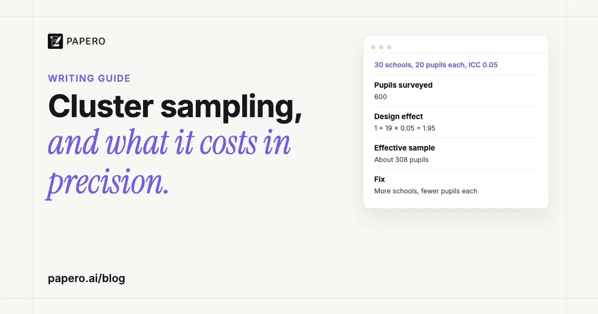
Cluster sampling is a probability sampling method in which you split a population into existing groups, such as schools, villages or city blocks, pick some of those groups at random, and then measure everyone in them or a random subset. It saves travel and listing costs and pays for them in precision: 600 pupils drawn from 30 schools can carry the information of about 308 pupils drawn one by one, if pupils in a school are modestly alike (an ICC of 0.05).
Key Takeaways
- The unit drawn at random is a group, not a person. One-stage designs measure everyone in the chosen groups; two-stage and multistage designs sample again inside them.
- Strata should be alike inside; clusters should each look like a small copy of the population.
- People in one group tend to answer alike. The intraclass correlation (ICC) measures that, and the design effect, 1 + (m − 1) × ICC, says how much it inflates the variance.
- Sample size divided by the design effect gives the effective sample size. With 20 pupils per school and an ICC of 0.05, 600 pupils count as about 308.
- More, smaller clusters beat fewer, bigger ones, and the analysis has to use the cluster IDs.
What is cluster sampling?
A cluster sample is a random sample of groups rather than of individuals. You list the groups that make up the population, draw some of them at random, and collect data from the people inside the chosen groups. Every person still has a known chance of selection, so it is a probability method, but people enter the sample in bunches. Statisticians call the groups primary units and the people in them secondary units.
OpenStax’s Introductory Statistics defines it in two steps: “divide the population into clusters (groups) and then randomly select some of the clusters. All the members from these clusters are in the cluster sample.” Penn State’s STAT 506 notes name the two situations where the design earns its place: when “a good frame listing the population elements either is not available or is very costly to obtain, whereas a frame listing clusters is easily obtained”, and when “the cost of obtaining observations increases as the distance separating the elements increases.”
That random step is what separates it from convenience sampling, which takes whoever is easy to reach.
What are the types of cluster sampling?
There are three types, and they differ in what happens inside the chosen clusters. One-stage designs measure every member of each selected cluster. Two-stage designs draw a random sample of members inside each selected cluster. Multistage designs repeat the draw through more levels, such as counties, then blocks, then households, then people, which is how the US NHANES health survey works.
| Type | Drawn at random | Who is measured | Example | Trade-off |
|---|---|---|---|---|
| One-stage | Clusters | Everyone in each chosen cluster | 30 schools, every pupil tested | Simplest; large clusters push the design effect up |
| Two-stage | Clusters, then members | A random subset of each chosen cluster | 30 schools, 20 pupils drawn in each | Fixes cluster size; needs a list only inside chosen clusters |
| Multistage | Units at three or more levels | People at the last stage | Counties, blocks, households, people | Fits national surveys; needs survey software |
Penn State’s lesson on multistage designs, which counts two-stage sampling as the simplest multistage design, cites a Gallup poll that samples about 300 election districts and then 5 households in each. When clusters differ a lot in size, they are often drawn with probability proportional to size (PPS), so a large county is more likely to be picked than a small one.
Cluster vs stratified sampling: what is the difference?
Both split the population into groups, but they use the groups in opposite ways. Stratified sampling takes people from every group, so it wants groups that are alike inside and different from each other, and it usually gains precision. A cluster design takes only some groups, so it wants each group to be a small, varied copy of the population, and it usually loses precision.
| Feature | Stratified sample | Cluster sample |
|---|---|---|
| Groups sampled | All of them | A random few |
| Who is measured | A random sample in every stratum | Everyone, or a random sample, in the chosen clusters |
| Ideal group | Alike inside, different from the others | Varied inside, each like the others |
| Usual effect on precision | Smaller standard errors than a simple random sample | Larger standard errors |
| Main reason to use it | Precision and subgroup estimates | Cost, or no list of individuals |
Penn State’s notes state both sides. For strata, look for “opportunities when the measurements within the strata are more homogeneous.” For clusters, “Clusters should be formed so that one cluster is similar to another cluster,” which “is very different from saying that units in the cluster are similar.”
Natural clusters rarely behave that well: Killip, Mahfoud and Pearce note that patients of one physician can share “geographic, socioeconomic, racial, ethnic, sexual, religious, political, or age-related similarities”. The two designs are also combined: NHANES sorts its counties into strata before drawing them. Our guide to stratified sampling covers the other column of the table.
Why is a cluster sample cheaper but less precise?
People in the same cluster resemble each other, so each extra person from a cluster you have already sampled adds less new information than a person drawn from anywhere in the population. You save on travel and on building lists, but the variance of your estimates grows. The intraclass correlation measures the resemblance, and the design effect turns it into lost sample size.
Penn State’s notes are blunt: “Will it give us a more precise estimator? The answer is no in most cases.” The design pays off when reaching people inside a cluster costs much less than reaching scattered individuals.
Killip and colleagues define the intracluster correlation coefficient (the ICC, which they write as ρ) as “the between-cluster variability divided by the sum of the within-cluster and between-cluster variabilities.” At 0, people in a cluster are no more alike than strangers; at 1, “all responses within a cluster are identical”, and the effective sample size falls to the number of clusters. They put typical values in human studies at 0.01 to 0.02. For clusters of equal size:
- Design effect (DEFF) = 1 + (m − 1) × ICC, where m is the number of people per cluster.
- Effective sample size = n ÷ DEFF, where n is the total number of people measured.
Killip’s case study shows the cost. Four physicians each recruited 32 patients, 128 in all, and with ρ = 0.017 the design effect is 1 + 31 × 0.017 = 1.527. The effective sample size is 84, which is why the trial’s power came out at 61% instead of the planned 80%.
Worked example: 30 schools, 20 pupils each
Survey 20 pupils in each of 30 randomly chosen schools, 600 pupils in all, and assume an ICC of 0.05 for the outcome. The design effect is 1 + (20 − 1) × 0.05 = 1.95. The effective sample size is 600 ÷ 1.95 ≈ 308, so the clustered sample is about as precise as 308 pupils drawn at random from the whole population.
The ICC here is an assumption; in a real study it comes from a pilot or from published studies of the same outcome. The steps, ignoring the finite population correction:
- Design effect: 1 + 19 × 0.05 = 1.95.
- Effective sample size: 600 ÷ 1.95 = 307.7, about 308 pupils.
- Standard errors grow by √1.95 ≈ 1.40, so confidence intervals are about 40% wider.
- For a proportion near 50%, the 95% margin of error with 600 independent pupils is 1.96 × √(0.25 ÷ 600) ≈ 4.0 percentage points. With the clustering it is 4.0 × 1.40 ≈ 5.6 points. An analysis that ignores the schools prints ±4.0 when the honest figure is ±5.6.
- To match 600 independent pupils at 20 per school, you need 600 × 1.95 = 1,170 pupils, or 58.5 schools: round up to 59 schools.
The same 600 pupils, split differently, give very different precision:
| Schools | Pupils per school | Design effect | Effective sample size |
|---|---|---|---|
| 15 | 40 | 2.95 | 203 |
| 30 | 20 | 1.95 | 308 |
| 60 | 10 | 1.45 | 414 |
| 120 | 5 | 1.20 | 500 |
The ICC matters as much as the split: at 20 pupils per school, an ICC of 0.01 gives a design effect of 1.19 (504 effective pupils) and 0.20 gives 4.80 (125). Killip and colleagues draw the rule from their own tables: “Increasing the number of clusters enhances power more efficiently than does increasing the number of subjects within a cluster.” Each extra school costs a visit, so a real design balances the cost per school against the cost per pupil.
Some explainers say this design weakens a study’s validity. That mixes up two problems. A random draw of schools, analysed with the right selection weights, gives unbiased estimates; what it costs is noise, a question of precision. The error that does the damage is analysing the pupils as if they had been drawn one by one, which makes the noise look smaller than it is. Our guide to reliability and validity separates the two ideas for measurement.
A real example: how NHANES uses multistage cluster sampling
The US National Health and Nutrition Examination Survey (NHANES) samples in four stages: counties (or parts or groups of counties), census blocks within them, households, then people. Its mobile examination centres travel to each sampled area, so clustering keeps the survey affordable. The cost is that each two-year sample comes from only 30 areas, and analysts must use the survey’s design variables to get honest standard errors.
What they did. The 2015–2018 design report by Chen and colleagues lists the stages: “(a) PSUs (counties, groups of tracts within counties, or combinations of adjacent counties), (b) segments within PSUs (census blocks or combinations of blocks), (c) dwelling units (DUs) (households) within segments, and (d) individuals within households.” The PSUs were grouped into 14 major strata with 4 minor strata each and drawn with PPS, apart from 4 taken with certainty. Each year 15 PSUs formed a nationally representative sample, and 24 segments were sampled in each noncertainty PSU.
The numbers. Over 2015–2018, 31,538 people were selected, 19,225 interviewed and 18,248 examined (the report’s Table I). NCHS’s variance tutorial gives the reason for so few areas: the survey “can only sample 30 Primary Sampling Units (PSUs) within a 2-year survey cycle because of operational limitations such as the cost of moving the survey MECs and geographic distances between PSUs.”
What it means for analysis. The report is direct: “Standard statistical software routines that assume a simple random sample should not be used for computing variances for NHANES.” Public files carry masked design variables, sdmvstra (pseudo-stratum) and sdmvpsu (pseudo-PSU), plus sample weights, and NCHS recommends Taylor series linearization in SUDAAN, Stata, R or SAS survey procedures. NCHS’s variance estimation tutorial adds that degrees of freedom are the number of PSUs minus the number of strata (15 for most two-year cycles), far fewer than the number of people.
What it can and cannot conclude. NHANES supports national estimates for the noninstitutionalized civilian population of the 50 states and the District of Columbia; US territories are not in the sample. With 30 PSUs per cycle, the report warns that “direct design-based variance estimates may be unstable for some measures” and that some subgroup samples are small. Combining cycles helps, the report says, “particularly for analysis of rare events and small subgroups.”
How do you analyse and report a cluster sample?
Keep the cluster ID, and any strata and weights, for every respondent, and analyse with survey methods that use them, such as Taylor series linearization or replication. Then report how many clusters you drew and how, how many people per cluster, the ICC or design effect you planned with, and the software and variance method you used.
Killip and colleagues add that the effective sample size “should be used to calculate power in the design phase of a clustered study”, so the planned ICC and its source belong in the write-up too. Our guide on how to write a methodology section shows where each item goes. If you ended up with few clusters, say so when you write up the limitations of your study: intervals will be wide and variance estimates unstable.
What are the advantages and disadvantages of cluster sampling?
The advantages are practical: you need a list of clusters rather than of every person, and fieldwork is concentrated in a few places. The disadvantages are statistical: a larger variance for the same number of people, analysis that needs the design variables, and unstable estimates when clusters are few.
In trials, Killip and colleagues add a further reason: randomising whole clusters avoids contamination, because patients of one physician may know each other and a counselled patient could pass the advice to one meant to get none. They also warn that accounting for clustering “almost always results in a net loss of power, requiring increased total subject recruitment.”
Where Papero fits
The ICC this design depends on comes from a pilot study or from published studies of the same outcome. Killip and colleagues note that estimating it “usually requires a pilot study” and ask researchers to publish their values. Papero’s Find papers page searches 250M+ papers through OpenAlex, so you can look for studies that measured your outcome in schools, clinics or villages and report an ICC or design effect, then save them to your source library.
Papero does not compute design effects or sample sizes; that part is yours. The glossary entry on what sample size means covers the basics, and the thesis writing page shows how chapter outlines, one source library and Review fit together.
Frequently Asked Questions
What is cluster sampling in simple terms?
It is a way of drawing a random sample by picking whole groups, such as schools or villages, instead of individual people, then surveying everyone in the chosen groups or a random subset. It is cheaper than drawing people one by one, but less precise for the same number of people.
Is cluster sampling a probability sampling method?
Yes. The clusters are chosen at random, and people inside them are either all included or drawn at random, so every member of the population has a known, nonzero chance of selection. That separates it from convenience or quota sampling. Because people in one cluster tend to be alike, the analysis has to account for the clusters to get correct standard errors.
What is the difference between cluster and stratified sampling?
Stratified sampling samples from every group; a cluster design samples only some groups. Strata work best when they are alike inside and usually make estimates more precise. Clusters work best when each is a varied, small copy of the population, and they usually make estimates less precise but cheaper to collect.
What is an example of cluster sampling?
A study of reading levels draws 30 schools at random from a region’s list of schools and tests 20 pupils in each; the schools are the clusters. A national example is the US National Health and Nutrition Examination Survey, which draws counties, then census blocks, then households, then people, from only 30 county-level units in each two-year cycle.
How do you calculate the design effect?
For clusters of equal size, the design effect is 1 + (m − 1) × ICC, where m is the number of people per cluster and ICC is the intraclass correlation of the outcome. Divide the total sample by the design effect to get the effective sample size. With 20 people per cluster and an ICC of 0.05, the design effect is 1.95, and 600 people count as about 308.
Sources
- Illowsky, B., & Dean, S. (2023). Introductory statistics 2e, Section 1.2, Data, sampling, and variation in data and sampling. OpenStax. https://openstax.org/books/introductory-statistics-2e/pages/1-2-data-sampling-and-variation-in-data-and-sampling
- Penn State Eberly College of Science. “6 Part A: Stratified Sampling.” STAT 506: Sampling Theory and Methods (online.stat.psu.edu, November 2026): https://online.stat.psu.edu/stat506/Lesson06.html
- Penn State Eberly College of Science. “7 Part 1 of Cluster and Systematic Sampling.” STAT 506: Sampling Theory and Methods (online.stat.psu.edu, November 2026): https://online.stat.psu.edu/stat506/Lesson07.html
- Penn State Eberly College of Science. “9 Multi-Stage Designs.” STAT 506: Sampling Theory and Methods (online.stat.psu.edu, November 2026): https://online.stat.psu.edu/stat506/Lesson09.html
- Killip, S., Mahfoud, Z., & Pearce, K. (2004). What is an intracluster correlation coefficient? Crucial concepts for primary care researchers. Annals of Family Medicine, 2(3), 204–208. https://doi.org/10.1370/afm.141
- Chen, T. C., Clark, J., Riddles, M. K., Mohadjer, L. K., & Fakhouri, T. H. I. (2020). National Health and Nutrition Examination Survey, 2015−2018: Sample design and estimation procedures (Vital and Health Statistics, Series 2, No. 184). National Center for Health Statistics. https://www.cdc.gov/nchs/data/series/sr_02/sr02-184-508.pdf
- National Center for Health Statistics. “Variance estimation.” NHANES Tutorials (wwwn.cdc.gov, November 2026): https://wwwn.cdc.gov/nchs/nhanes/tutorials/VarianceEstimation.aspx