A cross-sectional study measures the exposure and the outcome in a group of people at the same moment, with no follow-up. It answers “how common is this?” (prevalence) and “what goes with it?” (association), but because nothing is measured before anything else, it cannot show which came first. Below: a worked 2x2 table, a national survey taken apart step by step, and how to report one.
Key Takeaways
- The design takes one snapshot. Participants are chosen by eligibility criteria, not by exposure (as in a cohort) or by outcome (as in a case-control study).
- Descriptive versions report prevalence; analytical versions compare the outcome between exposed and unexposed people.
- For associations, the prevalence ratio is easier to read than the odds ratio, which overstates it when the outcome is common: 2.43 against 2.0 in the worked example below.
- Temporality is the built-in limit. A link between X and Y in one survey fits X causing Y, Y causing X, or a third factor causing both.
- Report it with the STROBE checklist for cross-sectional studies: 22 items, starting with naming the design in the title or abstract.
What is a cross-sectional study?
A cross-sectional study is an observational design in which researchers select a sample from a population and record, at one point in time, both the exposures and the outcomes of each participant. Nobody is assigned to a treatment and nobody is followed up, so the data describe the population as it was on the day of measurement.
Wang and Cheng, writing in Chest, put it this way: “investigators measure outcomes and exposures of the study subjects at the same time.” What sets the design apart is how people get in. Cohort studies select participants by exposure and case-control studies by outcome, while here they are “just selected based on the inclusion and exclusion criteria set for the study”, in Setia’s words. Exposure and outcome are then found among whoever was sampled, through questionnaires, interviews, examinations or routine records.
The design is common in published research. Barros and Hirakata counted the original articles published in 1998 in two journals, the International Journal of Epidemiology and Revista de Saúde Pública: 110 of 221 (50%) were cross-sectional. Our guide to types of research methodology shows where it sits among the observational designs.
How is a cross-sectional study different from longitudinal and cohort studies?
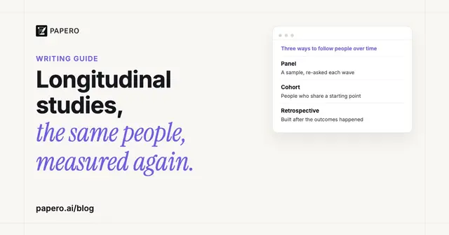
The difference is time. A cross-sectional design measures each person once. A longitudinal study measures the same people repeatedly, and a cohort study, one kind of longitudinal study, starts from people grouped by exposure and follows them forward to see who develops the outcome. A case-control study starts from people who already have the outcome and looks back at their exposures.
| Design | How participants are chosen | When things are measured | Main measure | What it shows about time order |
|---|---|---|---|---|
| Cross-sectional | By eligibility criteria only | Exposure and outcome together, once | Prevalence; prevalence ratio or odds ratio | Nothing: both are measured at once |
| Repeated cross-sectional | A new sample from the same population each round | Once per person, several rounds | Change in prevalence across rounds | Change in the population, not in individuals |
| Longitudinal (panel) | One sample, kept | The same people, several times | Change within each person | Which changes came first in each person |
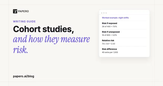
| Cohort | By exposure status | Exposure first, outcome after follow-up | Incidence; relative risk | Exposure is recorded before the outcome |
| Case-control | By outcome status | Outcome first, past exposure recalled or looked up | Odds ratio | Depends on how well past exposure is recorded |
The repeated cross-sectional row causes the most confusion. A national survey repeated every year or two with a fresh sample shows how a population changes, but Wang and Cheng are explicit that such surveys “cannot be used to look at individual change (as in a cohort study).” Our guides to the longitudinal study and the cohort study cover both designs in depth.
Descriptive vs analytical cross-sectional studies
A descriptive cross-sectional study counts: what share of a defined population has a condition, an attitude or a behaviour. An analytical one also compares: it splits the sample by an exposure and asks whether the outcome is more common in one group. Many studies do both, reporting prevalence first and associations second; the UK Faculty of Public Health’s textbook notes that in practice they “often include an element of both types of design.”
Wang and Cheng give a published example of each variant:
- Descriptive. Thomas and colleagues sent a breathing questionnaire to 307 adults treated for asthma in one general practice; 227 returned it (74%), and about one third of women and one fifth of men scored in the range suggesting dysfunctional breathing.
- Analytical. Janson and colleagues analysed 7,882 never-smokers from 36 centres in 16 countries and found passive smoking was associated with nocturnal chest tightness, breathlessness and increased bronchial responsiveness.
- Repeated. Soriano and colleagues compared Spanish surveys of 4,030 adults in 1997 and 3,802 in 2007: COPD prevalence fell from 9.1% to 4.5%, a population trend in which no single adult was measured twice.
What does a cross-sectional study measure?
The core measure is prevalence: the share of people who have the outcome at the time of the survey, whenever it began. Incidence, the number of new cases over a period, needs follow-up and is out of reach. For an association, the analysis compares prevalence in the exposed group with prevalence in the unexposed group, as a ratio (prevalence ratio) or through odds (odds ratio).
Prevalence depends on how many people develop the outcome and on how long they live with it; Setia notes that HIV prevalence can rise even while new infections fall. The Faculty of Public Health textbook draws the consequence: because these studies count existing cases, “the data will always reflect determinants of survival as well as aetiology.”
The choice of ratio is where many reports go wrong. Logistic regression produces odds ratios, and in Barros and Hirakata’s 1998 sample it was used in 37 of the 110 cross-sectional articles (34%). They argue that in this design “the odds ratio can importantly overestimate the prevalence ratio, the measure of choice in these studies”, and recommend models that estimate the prevalence ratio directly: log-binomial regression, or Poisson regression with sandwich variance estimates. We side with them for any outcome that is not rare, for a practical reason: readers interpret every ratio as “times as likely”, and only the prevalence ratio means that.
Worked example: prevalence and a prevalence ratio from a 2x2 table
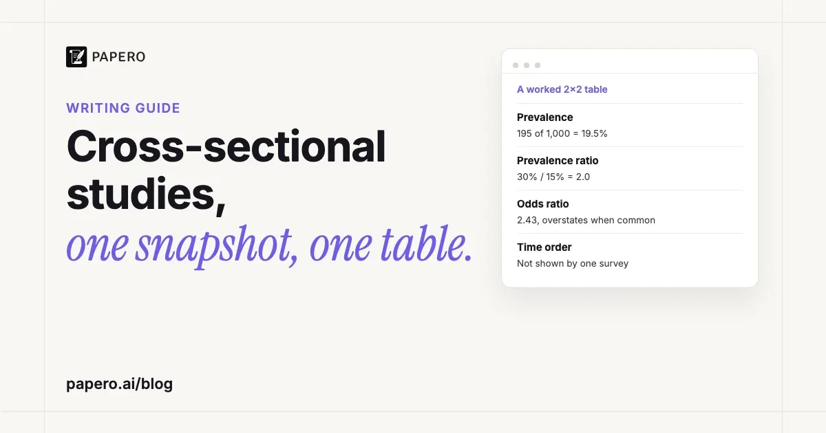
The numbers here are invented. A university surveys 1,000 undergraduates in one week of term. The exposure is sleeping under six hours on most weeknights (300 students say yes). The outcome is screening positive on a depression questionnaire (195 students do). The 2x2 table crosses the two:
| Screened positive | Screened negative | Total | Prevalence | |
|---|---|---|---|---|
| Short sleep (exposed) | 90 (a) | 210 (b) | 300 | 90 / 300 = 30.0% |
| Adequate sleep (unexposed) | 105 (c) | 595 (d) | 700 | 105 / 700 = 15.0% |
| Total | 195 | 805 | 1,000 | 195 / 1,000 = 19.5% |
Prevalence. Overall prevalence is 195 / 1,000 = 19.5%. That single number is the descriptive result.
Prevalence ratio (PR). Divide the two group prevalences: 30.0% / 15.0% = 2.0. Short sleepers are twice as likely to screen positive at the time of the survey. With the usual log-based formula, the 95% confidence interval runs from 1.56 to 2.56.
Prevalence odds ratio (OR). Odds are cases divided by non-cases: 90 / 210 = 0.429 in the exposed group and 105 / 595 = 0.176 in the unexposed group. Their ratio, (a × d) / (b × c) = (90 × 595) / (210 × 105) = 53,550 / 22,050, is 2.43.
The two measures disagree because the outcome is common. If only 2% of short sleepers (6 of 300) and 1% of the others (7 of 700) screened positive, the prevalence ratio would still be 2.0 and the odds ratio would be 2.02. At 15% and 30%, reading the odds ratio as “2.4 times as likely” makes the ratio about a fifth larger than it is (2.43 against 2.0). Setia’s teaching table shows the same pattern: 50 of 200 men and 10 of 100 women with HIV give an odds ratio of 3.0, while the prevalence ratio from that table is 2.5.
What the table cannot tell you is the direction. Students with depressive symptoms might sleep badly because of those symptoms, or short sleep might feed them, and one survey cannot separate the two.
Why can’t a cross-sectional study show cause and effect?
A causal claim needs the cause to come before the effect, and a single survey records both at once. An association between exposure and outcome fits at least three stories: the exposure raised the outcome, the outcome changed the exposure (reverse causation), or a third factor drove both (confounding). Setia’s summary is that “it is difficult to derive causal relationships from cross-sectional analysis.”
Setia’s own example of reverse causation is worth remembering. Survey 250 people on diet, exercise and body mass index, and you may find that people with obesity eat more salads and exercise more. The salads did not cause the weight; people changed their habits after gaining it. Measured on one day, habit and weight look like cause and effect running the wrong way.
Measuring existing cases brings two more biases. People whose illness was brief or fatal are missing from the sample, a form of what Wang and Cheng list as prevalence-incidence (Neyman) bias: the exclusion of people with severe or mild disease. Questions about past exposure invite recall bias, because people who already have the outcome remember differently. Confounding is handled as in any observational design, by restriction, stratification, matching or regression; our guide to confounding variables shows a published case where a confounder reversed a result. Adjustment does nothing for temporality, though: the direction problem stays in a perfectly adjusted model.
A real example: social media use and sadness in the 2023 YRBS
CDC’s Youth Risk Behavior Survey (YRBS) is a cross-sectional survey of US high school students, run every two years since 1991 with a new nationally representative sample each time. In 2023 it asked, for the first time, how often students use social media. Young and colleagues analysed the answers against bullying, persistent sadness and suicide risk in an open-access MMWR report.
What they did. The survey had 20,103 usable questionnaires from grades 9 to 12. “Frequent social media use” meant using it at least several times a day. Outcomes were yes/no answers about the past 12 months. The authors estimated prevalence with survey weights and compared groups with prevalence ratios, adjusted for age, race and ethnicity, sex and sexual identity.
The numbers. Overall, 77.0% of students reported frequent use (81.8% of female and 72.9% of male students). Persistent feelings of sadness or hopelessness were reported by 42.6% of frequent users and 31.9% of less frequent users: a prevalence ratio of 1.33 (95% CI 1.07 to 1.65), and 1.35 (1.23 to 1.47) after adjustment. Attempted suicide showed no difference: 9.5% in both groups, adjusted PR 1.11 (0.89 to 1.39). The worked-example method checks the first ratio: 42.6 / 31.9 = 1.34, the published 1.33 within rounding.
What it can conclude. How common frequent social media use was among US high school students in 2023, and that sadness was about a third more common among frequent users, a gap that held when four demographic factors were accounted for.
What it cannot conclude. That social media causes sadness. The authors write: “YRBS data are cross-sectional; causality and directionality of associations between frequent social media use and health behaviors and experiences cannot be established.” Sad or lonely teenagers spending more time online would produce the same table. Three further limits sit in the report and its methods overview:
- Only 15,203 of the 20,103 respondents answered the social media question, so about a quarter of the sample is missing from the exposure.
- The “less frequent” group combines students who never use social media with daily users, which the authors say “might” mask differences.
- The overall response rate was 35.4%, “the lowest in the history of the survey”, and teenagers not in school are outside the sample.
Taken together, the report’s limits make a model for your own: each is specific, carries a number, and the direction problem is stated outright. Our guide to the limitations of a study shows how to write one for your own project.
What are the strengths and weaknesses of cross-sectional studies?
The strengths are speed, cost and breadth: one round of data collection, no follow-up, several exposures and outcomes at once, and the best available estimate of prevalence. The weaknesses come from the same single snapshot: no incidence, no time order, a poor fit for rare or short-lived conditions, and exposure to non-response and recall bias.
Because no one is deliberately exposed or treated, Wang and Cheng note, “there are seldom ethical difficulties”, one reason the design suits student research with limited time. Questionnaires reach large samples cheaply but “can result in low response rates”, so sampling carries most of the weight; our guide to stratified sampling explains one way survey samples are built. A cross-sectional survey is often the first study on a question: Setia notes it is run before planning a cohort study, or as a cohort’s baseline, where its prevalence figures help design what follows.
How do you report a cross-sectional study?
Follow the STROBE checklist for cross-sectional studies, the reporting guideline written for the three main observational designs: cohort, case-control and cross-sectional. It has 22 items covering the title, introduction, methods, results, discussion and funding. Four of them (items 6, 12, 14 and 15) differ by design, in whole or in part. Six items deserve a second look in a cross-sectional report:
- Item 1a. “Indicate the study’s design with a commonly used term in the title or the abstract.” Write “a cross-sectional survey”, not “a survey”.
- Item 6a. Give the eligibility criteria and the sources and methods of selecting participants.
- Item 12d. “If applicable, describe analytical methods taking account of sampling strategy”, such as the survey weights in the YRBS example.
- Item 14b. Give the number of participants with missing data for each variable.
- Item 16a. Give unadjusted and adjusted estimates with their 95% confidence intervals, and say which confounders were adjusted for and why.
- Item 19. Discuss limitations, “both direction and magnitude of any potential bias.”
In the methods, name the design in the first sentence and justify it against the stronger design you could not run; our guide to the methodology section maps STROBE items to each subsection. In the discussion, use association verbs (“was associated with”, “was more common among”) and keep causal verbs (“led to”, “increased”) out.
Where Papero fits
Papero is an AI writing workspace for students and researchers. Its Find papers page searches more than 250 million papers through OpenAlex, so you can read published cross-sectional surveys on your topic and see how they word their limitations before you write yours. Among the Review checks, Claims finds sentences that need a citation and offers papers to cite, which helps with the background paragraph of a survey report.
Papero does not design your study or run your statistics; the 2x2 table above is yours to calculate. The glossary entry on research design defines the related terms, and the research paper writing page shows the outline-to-manuscript workflow.
Frequently Asked Questions
What is a cross-sectional study in simple terms?
It is a snapshot. Researchers measure a sample of people once, at the same point in time, with no follow-up. The result shows how common something is and what tends to go with it, but not which came first, so it does not prove cause and effect.
What is an example of a cross-sectional study?
The US Youth Risk Behavior Survey is one. In 2023, 20,103 high school students answered one questionnaire; an analysis found that 77.0% used social media at least several times a day and that persistent sadness was more common among them (42.6% against 31.9%). Because both were measured at once, the authors state that causality and direction cannot be established.
Can cross-sectional studies show causation?
Not on their own. Exposure and outcome are measured at the same time, so the data fit the exposure causing the outcome, the outcome causing the exposure, or a third factor causing both. Statistical adjustment deals with measured confounders but not with time order, which needs a cohort study or a trial.
What is the difference between cross-sectional and longitudinal research?
Cross-sectional research measures each participant once. Longitudinal research measures the same participants several times, so it shows change within people and the order in which things happened. A repeated cross-sectional survey sits in between: it samples the same population at several points but draws new people each time, so it shows population trends, not individual change.
Should you report odds ratios or prevalence ratios?
Both are valid, but the prevalence ratio is easier to interpret. When the outcome is common, the odds ratio lies further from 1 than the prevalence ratio and is often misread as “times as likely”. Where 30% of exposed and 15% of unexposed people have the outcome, the prevalence ratio is 2.0 and the odds ratio 2.43. Log-binomial or Poisson regression estimates the prevalence ratio directly.
Sources
- Wang, X., & Cheng, Z. (2020). Cross-sectional studies: Strengths, weaknesses, and recommendations. Chest, 158(1, Suppl.), S65–S71. https://doi.org/10.1016/j.chest.2020.03.012
- Setia, M. S. (2016). Methodology series module 3: Cross-sectional studies. Indian Journal of Dermatology, 61(3), 261–264. https://doi.org/10.4103/0019-5154.182410
- Barratt, H., Kirwan, M., & Shantikumar, S. (2018). Design, applications, strengths and weaknesses of cross-sectional, analytical studies (including cohort, case-control and nested case-control studies), and intervention studies (including randomised controlled trials). In Health Knowledge public health textbook. Faculty of Public Health. https://www.healthknowledge.org.uk/public-health-textbook/research-methods/1a-epidemiology/cs-as-is
- Barros, A. J. D., & Hirakata, V. N. (2003). Alternatives for logistic regression in cross-sectional studies: An empirical comparison of models that directly estimate the prevalence ratio. BMC Medical Research Methodology, 3, Article 21. https://doi.org/10.1186/1471-2288-3-21
- Young, E., McCain, J. L., Mercado, M. C., Ballesteros, M. F., Moore, S., Licitis, L., Stinson, J., Everett Jones, S., & Wilkins, N. J. (2024). Frequent social media use and experiences with bullying victimization, persistent feelings of sadness or hopelessness, and suicide risk among high school students: Youth Risk Behavior Survey, United States, 2023. MMWR Supplements, 73(4), 23–30. https://doi.org/10.15585/mmwr.su7304a3
- Brener, N. D., Mpofu, J. J., Krause, K. H., Everett Jones, S., Thornton, J. E., Myles, Z., Harris, W. A., Chyen, D., Lim, C., Arrey, L., Mbaka, C. K., Trujillo, L., Shanklin, S. L., Smith-Grant, J., Whittle, L., McKinnon, I. I., Washington, M., Queen, B. E., & Roberts, A. M. (2024). Overview and methods for the Youth Risk Behavior Surveillance System: United States, 2023. MMWR Supplements, 73(4), 1–12. https://doi.org/10.15585/mmwr.su7304a1
- von Elm, E., Altman, D. G., Egger, M., Pocock, S. J., Gøtzsche, P. C., & Vandenbroucke, J. P. (2007). The Strengthening the Reporting of Observational Studies in Epidemiology (STROBE) statement: Guidelines for reporting observational studies. PLOS Medicine, 4(10), Article e296. https://doi.org/10.1371/journal.pmed.0040296
- STROBE. (n.d.). STROBE statement: Checklist of items that should be included in reports of cross-sectional studies. https://www.strobe-statement.org/download/strobe-checklist-cross-sectional-studies-pdf