
A cohort study is an observational design that starts with people who do not yet have an outcome, records who is exposed to a factor and who is not, and follows both groups to count who develops the outcome. Comparing the two groups gives the risk linked to the exposure. This guide works through a 2x2 example and the British Doctors Study, which followed 34,439 men for 50 years.
Key Takeaways
- People enter a cohort by exposure status and nobody has the outcome yet, so the exposure comes first in time.
- Prospective cohorts are followed forward from now; retrospective (historical) cohorts rebuild the comparison from existing records.
- The core results are the risk in each group, the relative risk (one risk divided by the other) and the risk difference (one minus the other).
- Person-time counts each participant only for the time they were watched, so people who drop out still contribute.
- The weak points are loss to follow-up, confounding that adjustment never fully removes, and the size and cost needed for rare outcomes.
What is a cohort study?
A cohort study is an observational study that selects people by their exposure, before any of them has the outcome, and follows them over time. The researcher does not assign the exposure: smoking, a job or a diagnosis is recorded as it already is. At the end, the groups are compared on how many new cases each produced. Because exposure is measured first, the design shows which came first.
The National Library of Medicine’s MeSH thesaurus defines cohort studies as “Studies in which subsets of a defined population are identified. These groups may or may not be exposed to factors hypothesized to influence the probability of the occurrence of a particular disease or other outcome.”
The word comes from the Latin cohors, “a group of soldiers”, as Setia explains in a methods series for clinicians. The defining rule is that “the participants do not have the outcome of interest to begin with.” Penn State’s epidemiology course (STAT 507) adds what the design is for: cohort studies “are useful for estimating disease risk, incidence rates, and/or relative risks.”
Setia notes that cohort studies are sometimes called prospective or longitudinal studies, although, as the next sections show, a cohort can also be built from past records. Our guide to longitudinal studies covers repeated measurement in general; this one stays with the exposed-versus-unexposed comparison.
Cohort vs case-control vs cross-sectional studies
The three observational designs differ in where they start. A cohort starts from exposure and waits for outcomes. A case-control study starts from the outcome, picking people who have it and people who do not, then looks back at their exposure. A cross-sectional study measures exposure and outcome at the same moment. Only the cohort measures risk directly, because only it counts new cases among people who were at risk.
| Feature | Cohort | Case-control | Cross-sectional |
|---|---|---|---|
| Starting point | Exposed and unexposed people, all free of the outcome | People with the outcome (cases) and without it (controls) | A sample of a population at one moment |
| Direction in time | Forward from exposure, in real time or through records | Backward from outcome to past exposure | None: one snapshot |
| Main measure | Risk, incidence rate, relative risk | Odds ratio | How common exposure and outcome are at that moment |
| Shows exposure came first | Yes | Weaker: exposure is recalled or looked up after the outcome | No |
| Efficient for | Rare exposures, several outcomes | Rare diseases, several exposures | Public health planning, quick estimates |
| Cost and time | Expensive, long-term | Less expensive, short-term | Low cost, short |
| Typical bias | Loss to follow-up | Recall bias | Over-counts long-lasting cases |
The cohort and case-control columns follow the comparison table in Penn State’s STAT 507 lesson on cohort studies; the cross-sectional column follows its lesson 7, which says that design “Cannot infer temporal sequence between exposure and disease”. The course ranks the designs too: a case-control study “offers less support for a causation hypothesis than the longer and more expensive cohort design”, but “stronger evidence than a cross-sectional study.”
The smoking evidence came from the two stronger designs, case-control first. Case-control studies of lung cancer from Western Europe and North America led in 1950 to the conclusion that smoking was “a cause, and an important cause” of the disease, and by 1954 the British Doctors Study had confirmed the excess of lung cancer among smokers prospectively. Our guide to the cross-sectional study covers the snapshot design in depth, and the decision path in our overview of types of research methodology shows where all three sit among other designs.
Prospective vs retrospective cohort studies
The two types differ in when the researcher arrives. In a prospective cohort, the researcher defines the group and measures exposure now, then follows people into the future. In a retrospective, or historical, cohort, exposure and outcomes are already in records such as employment files or clinical notes, and the researcher reconstructs the follow-up from them. Both still run from exposure to outcome.
| Prospective cohort | Retrospective cohort | |
|---|---|---|
| When exposure is measured | At the start of the study, by the researcher | Before the study began, by whoever kept the records |
| Where outcomes come from | Follow-up visits, questionnaires, registry links | Existing records |
| Speed and cost | Slow and costly: follow-up can take decades | Faster and cheaper |
| Main risk | Dropouts, loss of funding | Incomplete or inconsistent records |
| Example | Framingham Heart Study, started 1948 | 430 patients’ clinic files, analysed for survival |
Prospective. The Framingham Heart Study began in 1948 by recruiting 5,209 men and women aged 30 to 62 at entry from Framingham, Massachusetts, who had not yet developed overt symptoms of cardiovascular disease or had a heart attack or stroke. Penn State lists the challenges of such studies: loss to follow-up, differential nonresponse, loss of funding, and exposure measures that improve while the study runs.
Retrospective. Setia’s example is a clinic with records on about 430 people with HIV, followed for 3 months to 4 years, 33 of whom had died. Analysing survival from those records is a retrospective cohort. It is quick, but the measurements “may not be very accurate or according to our requirements”. Zabert, Patino and Ferreira add that historical designs “may suffer from incomplete data and biases such as misclassification of exposure or outcomes.”
A retrospective cohort is easy to confuse with a case-control study. Penn State’s test: a retrospective cohort “uses the entire cohort; all cases and non-cases within the identified group”, while a case-control study selects cases and then picks controls.
How does a cohort study measure risk?
It counts new cases in each group. Cumulative incidence, or risk, is the number of new cases divided by the number of people at risk at the start. The relative risk divides the exposed group’s risk by the unexposed group’s; 1.0 means no difference. The risk difference subtracts the unexposed risk from the exposed risk. When people are followed for different lengths of time, an incidence rate per person-time replaces the simple proportion.
CDC’s epidemiology course defines the incidence proportion as “the proportion of an initially disease-free population that develops disease, becomes injured, or dies during a specified (usually limited) period of time”, and lists risk and cumulative incidence as synonyms. A relative risk above 1.0 points to higher risk in the exposed group; below 1.0, the exposure may protect.
With the standard 2x2 layout (a and b are the exposed people with and without the outcome, c and d the unexposed):
- Risk in the exposed = a / (a + b)
- Risk in the unexposed = c / (c + d)
- Relative risk = risk in the exposed / risk in the unexposed
- Risk difference = risk in the exposed − risk in the unexposed
- Incidence rate = new cases / total person-time at risk
Person-time handles people who leave early. In Penn State’s words, the time each person contributes is “the time from study enrollment until becoming a case, or the time until study completion or dropping out of the study.” CDC describes the four end points of each person’s follow-up: onset of disease, death, migration out of the study (lost to follow-up), or the end of the study.
Worked example: night shifts and type 2 diabetes
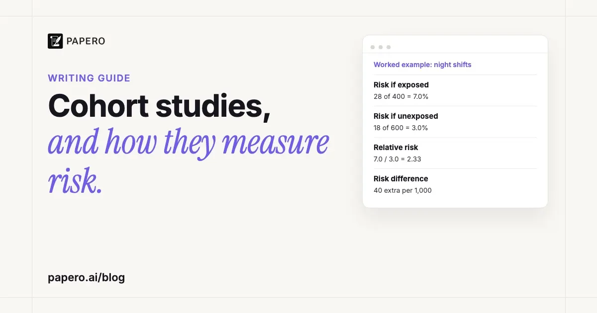
Here is a cohort we made up to show the arithmetic. A company enrols 1,000 employees without diabetes: 400 work night shifts and 600 work days. Over five years, 28 night workers and 18 day workers are diagnosed with type 2 diabetes. That is a five-year risk of 7.0% against 3.0%, a relative risk of 2.33 and a risk difference of 4 percentage points.
| Shift pattern | Developed diabetes | Did not | Total | Five-year risk |
|---|---|---|---|---|
| Night shifts (exposed) | a = 28 | b = 372 | 400 | 28 / 400 = 7.0% |
| Day shifts (unexposed) | c = 18 | d = 582 | 600 | 18 / 600 = 3.0% |
| Total | 46 | 954 | 1,000 | 46 / 1,000 = 4.6% |
- Relative risk = 0.070 / 0.030 = 2.33. Night workers were 2.33 times as likely to develop diabetes over five years.
- Risk difference = 0.070 − 0.030 = 0.040, or 40 extra cases per 1,000 night workers over five years.
- Turned around, 1 / 0.040 = 25: one more case for every 25 people on night shifts, if the difference were caused by the shifts.
The relative risk says how strongly the exposure is linked to the outcome; the risk difference says how many more cases the exposed group had, which is what a health service plans with once the link is judged causal. Report both.
Now add a fact the 2x2 hides. Not everyone stayed: 32 night workers and 42 day workers left the company, on average after 2 years, and the table above counted them as people who did not develop diabetes. CDC warns that this “assumes that they remained disease-free”. Person-time fixes it. Following CDC’s convention that a case diagnosed during a year counts half of that year, and assuming cases were diagnosed in year 3 on average, each case contributes 2.5 years here.
| Shift pattern | Cases | Left early | Completed 5 years | Person-years | Rate per 1,000 person-years |
|---|---|---|---|---|---|
| Night shifts | 28 × 2.5 = 70 | 32 × 2 = 64 | 340 × 5 = 1,700 | 1,834 | 28 / 1,834 = 15.3 |
| Day shifts | 18 × 2.5 = 45 | 42 × 2 = 84 | 540 × 5 = 2,700 | 2,829 | 18 / 2,829 = 6.4 |
The rate ratio is 15.27 / 6.36 = 2.40, and the rate difference is 8.9 cases per 1,000 person-years. The rate ratio sits close to the relative risk of 2.33 because the outcome is uncommon (7% and 3%) and the losses were similar in the two groups (8.0% of night workers, 7.0% of day workers). When losses are large or uneven between groups, the rate is the safer measure, since it counts only the time each person was observed.
What this cohort cannot tell you yet: whether night shifts cause diabetes. Night workers may be older, heavier, or smoke more, and each of those raises diabetes risk on its own. These are confounding variables, and until they are measured and adjusted for, 2.33 is a crude association. If the night workers who left were the ones already gaining weight, the loss to follow-up biases the result as well.
A real example: the British Doctors Study
The British Doctors Study is the classic prospective cohort. In 1951 a questionnaire on smoking went to every doctor in the UK whose address the British Medical Association knew, and their deaths were then tracked for 50 years. The 2004 report by Doll, Peto, Boreham and Sutherland covers 34,439 male doctors. Lifelong non-smokers died of lung cancer at 0.17 per 1,000 men a year, and continuing cigarette smokers at 2.49.
What they did. Two thirds of the doctors sent usable replies. Doctors were chosen partly because they “might take the trouble to describe their own smoking habits accurately”, but mainly because they had to stay on the medical register to practise, which made their deaths easy to trace. Smoking habits were asked again in 1957, 1966, 1971, 1978 and 1991. Richard Doll and Austin Bradford Hill published the first results in 1954.
How they handled follow-up. The authors withdrew 2,459 men living abroad in 1971, 467 who asked for no more questionnaires and 17 struck off the register. Among the remaining 31,496, follow-up of deaths was 99.2% complete, with 248 untraced, and 25,346 had died by 2001. Men who were withdrawn or untraced counted in the analysis until the time of withdrawal or last contact: person-time in practice.
The numbers. Table 1 of the paper gives death rates per 1,000 men per year, standardised for age and study period. The ratios and differences in the last two columns are our arithmetic from those rates.
| Cause of death | Lifelong non-smokers | Current cigarette smokers | Rate ratio (ours) | Extra deaths per 1,000 a year (ours) |
|---|---|---|---|---|
| Lung cancer | 0.17 | 2.49 | 14.6 | 2.32 |
| Lung cancer, 25 or more cigarettes a day | 0.17 | 4.17 | 24.5 | 4.00 |
| Ischaemic heart disease | 6.19 | 10.01 | 1.6 | 3.82 |
| External causes (accidents, injury, poisoning) | 0.71 | 1.13 | 1.6 | 0.42 |
| All causes | 19.38 | 35.40 | 1.8 | 16.02 |
Lung cancer has by far the highest ratio, but heart disease adds more deaths, 3.82 against 2.32 per 1,000 men a year, because it is so much more common. The authors found that a quarter of the excess deaths among smokers came from lung cancer and chronic obstructive lung disease, and another quarter from ischaemic heart disease. The lung cancer rate also climbs with dose, from 1.31 at 1 to 14 cigarettes a day to 2.33 at 15 to 24 and 4.17 at 25 or more.
The headline: men born in 1900 to 1930 who kept smoking cigarettes “died on average about 10 years younger than lifelong non-smokers”, and stopping at 60, 50, 40 or 30 gained about 3, 6, 9 or 10 years of life expectancy.
What it can and cannot conclude. Exposure was recorded decades before death, the follow-up was nearly complete, and risk rose with the number of cigarettes, so the link between smoking and these deaths is hard to dismiss. The external-causes row is a warning, though. The authors judged that excess “unlikely to be due chiefly to smoking” and put it down instead to “other behavioural factors with which smoking is associated, such as the heavy consumption of alcohol or a willingness to take risks.” That is confounding showing up in the data. The cohort was also men only and doctors only, and for the case that the differences are causal the authors point to their earlier reports, not to this table alone.
Strengths and weaknesses of cohort studies
The strengths come from measuring exposure first: the time order is clear, one exposure can be followed to many outcomes, and risk is measured directly. The weaknesses come from waiting. People drop out, follow-up costs years and money, rare outcomes need very large groups, and because nobody assigns the exposure, confounding is always possible. A retrospective design trades the waiting for older, less complete data.
Strengths. Setia lists temporality first: because nobody has the outcome at entry, “the temporality between exposure and outcome is well defined”. One exposure can be linked to several outcomes, as smoking was to lung cancer, heart disease and all-cause death. A cohort is efficient for a rare exposure, and can even suit a rare outcome when the exposed are at high risk: to study a chemical suspected of causing melanoma, Setia suggests following people exposed to it, at work or otherwise. Measuring habits before anyone is ill also cuts recall bias.
Weaknesses.
- Loss to follow-up. Setia warns that if more than 30% of a cohort is lost, “the validity of the results from this study are doubtful”, and it matters most when the people lost differ by exposure or outcome.
- Confounding. Exposed people choose or fall into their exposure, so they differ in other ways. Zabert and colleagues note that even after adjustment “there is always a risk of unmeasured or residual confounding.”
- Rare outcomes. Penn State’s comparison table lists “A large sample size often required, especially for rare outcomes” as a cohort drawback; a case-control design is usually preferred there.
- Misclassification. If exposure is recorded wrongly at random, Setia explains, the estimate is biased toward no effect, so the true association is underestimated.
Name each weakness in your discussion, with the direction it would push the result; our guide to writing the limitations of a study shows how.
How to write up a cohort study
Report the cohort so a reader can check every step: who was eligible, how exposure was measured, how long people were followed, how many were lost and why, the outcome events in each group, and both relative and absolute results with the confounders you adjusted for. Health journals expect the STROBE checklist of 22 items, four of them specific to the design.
Von Elm and colleagues write that 18 STROBE items “are common to all three study designs and four are specific for cohort, case-control, or cross-sectional studies.” Our guide to the methodology section maps the STROBE items that belong in methods.
For the worked example, a results sentence reads: “Over five years, 28 of 400 night-shift workers (7.0%) and 18 of 600 day-shift workers (3.0%) developed type 2 diabetes (crude relative risk 2.33; risk difference 4.0 percentage points). Seventy-four participants (7.4%) left before the end of follow-up.” Give the counts behind every percentage and label crude and adjusted estimates.
Where Papero fits
Papero does not design your study or run the statistics; the risk tables stay with you and your analysis software. It helps with the reading and writing around a cohort: finding published cohorts on your exposure, keeping them in one library, and citing them in your methods and discussion.
Find papers searches more than 250 million papers through OpenAlex and saves any result to your source library. Upload the PDFs and chat answers questions about them, citing the passages it used, which helps when you check how a published cohort defined exposure or handled dropouts. When the draft is done, the Review Claims check finds sentences that still need a citation and offers papers to cite, and every citation formats in APA 7 or eight other styles. The literature review workflow shows how these fit together, and the glossary entry on research design places cohorts among the other designs.
Frequently Asked Questions
Is a cohort study qualitative or quantitative?
It is quantitative. The design counts new cases of an outcome in exposed and unexposed groups and compares them as risks, rates, relative risks and risk differences. The comparison between exposure groups, which defines the design, rests on counts and rates rather than on interviews or observation notes.
What is the difference between a cohort and a case-control study?
A cohort starts with people who do not have the outcome, groups them by exposure and follows them to see who develops it, so it measures risk directly. A case-control study starts with people who already have the outcome and a comparison group without it, then looks back at exposure, and it estimates an odds ratio. Case-control studies are faster and suit rare diseases; cohorts show the time order more clearly.
Can a cohort study prove causation?
Not on its own. A cohort shows that the exposure came before the outcome, which a cross-sectional study cannot, but the exposed and unexposed groups were not formed at random, so a confounder can explain part or all of the difference. Strong, dose-dependent associations with nearly complete follow-up, such as the rise in lung cancer deaths with cigarettes smoked per day among 34,439 British doctors followed for 50 years, make a causal reading more convincing, especially when other designs agree.
What does a relative risk of 2 mean in a cohort study?
It means the exposed group developed the outcome twice as often as the unexposed group over the same follow-up period. A relative risk of 1.0 means no difference, and below 1.0 the exposure is linked to lower risk. The relative risk says nothing about how common the outcome is, so report the risk difference too: doubling a 1 in 10,000 risk adds far fewer cases than doubling a 1 in 10 risk.
Sources
- Doll, R., Peto, R., Boreham, J., & Sutherland, I. (2004). Mortality in relation to smoking: 50 years’ observations on male British doctors. BMJ, 328(7455), 1519. https://doi.org/10.1136/bmj.38142.554479.AE
- Doll, R., & Hill, A. B. (2004). The mortality of doctors in relation to their smoking habits: A preliminary report (Reprinted from British Medical Journal, 1954). BMJ, 328(7455), 1529–1533. https://doi.org/10.1136/bmj.328.7455.1529
- Setia, M. S. (2016). Methodology series module 1: Cohort studies. Indian Journal of Dermatology, 61(1), 21–25. https://doi.org/10.4103/0019-5154.174011
- Zabert, G., Patino, C. M., & Ferreira, J. C. (2025). Prospective cohort studies and their contribution to public health end [sic] evidence-based medicine. Jornal Brasileiro de Pneumologia, 51(4), Article e20250355. https://doi.org/10.36416/1806-3756/e20250355
- von Elm, E., Altman, D. G., Egger, M., Pocock, S. J., Gøtzsche, P. C., & Vandenbroucke, J. P. (2007). The Strengthening the Reporting of Observational Studies in Epidemiology (STROBE) statement: Guidelines for reporting observational studies. PLOS Medicine, 4(10), Article e296. https://doi.org/10.1371/journal.pmed.0040296
- National Library of Medicine. (n.d.). Cohort studies. In Medical Subject Headings (MeSH) (ncbi.nlm.nih.gov, November 2026). https://www.ncbi.nlm.nih.gov/mesh/?term=Cohort+Studies
- Penn State Eberly College of Science. (n.d.). Lesson 6: Cohort studies. In STAT 507: Epidemiological research methods (online.stat.psu.edu, November 2026). https://online.stat.psu.edu/stat507/Lesson06
- Penn State Eberly College of Science. (n.d.). Lesson 5: Case control studies. In STAT 507: Epidemiological research methods (online.stat.psu.edu, November 2026). https://online.stat.psu.edu/stat507/Lesson05
- Penn State Eberly College of Science. (n.d.). Lesson 7: Other types of study designs: Cross-sectional, ecologic, experimental. In STAT 507: Epidemiological research methods (online.stat.psu.edu, November 2026). https://online.stat.psu.edu/stat507/Lesson07
- Centers for Disease Control and Prevention. (2012). Lesson 3: Measures of risk, sections 2 and 5. In Principles of epidemiology in public health practice (3rd ed.). CDC archive (archive.cdc.gov, November 2026): https://archive.cdc.gov/www_cdc_gov/csels/dsepd/ss1978/lesson3/section2.html