Stratified sampling divides a population into non-overlapping groups, called strata, and draws a separate random sample from each one. Because every group is sampled, none can be left out by chance, and when the groups differ from each other the estimate is more precise than a simple random sample of the same size. This guide covers the steps, proportional versus Neyman allocation, and a worked example with the numbers shown.
Key Takeaways
- Strata are non-overlapping groups defined before sampling, using a variable you already know for every unit, such as year of study, region or type of school.
- Proportional allocation samples every stratum at the same rate. Neyman (optimal) allocation gives more of the sample to strata that are larger and more variable.
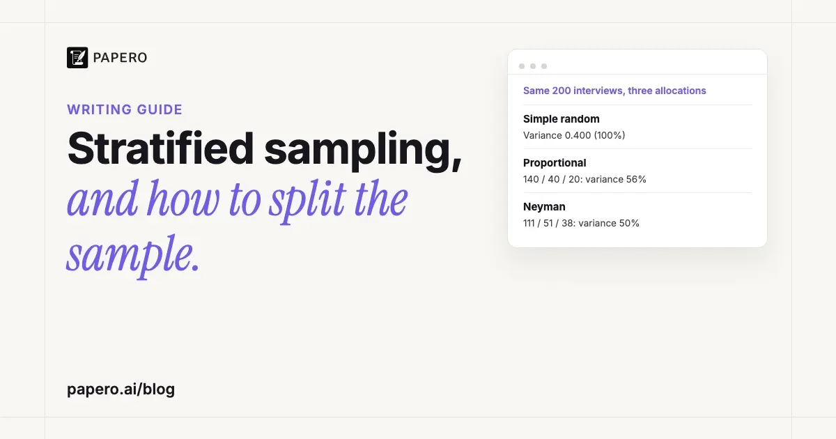
- In our worked example (2,000 students, a sample of 200), proportional allocation cut the variance of the estimated mean by 44% and Neyman allocation by 50%, compared with a simple random sample of the same size.
- Stratifying on a variable unrelated to the outcome buys no precision. In a Penn State course example, the stratified confidence interval came out wider.
- Stratified designs sample within every group; cluster designs sample whole groups. CDC’s Youth Risk Behavior Survey uses both.
What is stratified sampling?
Stratified sampling is a probability sampling method: you split the population into non-overlapping groups (strata), then select a sample inside each group by a random design. When that design is a simple random sample in every stratum, the result is called a stratified random sample. The strata results are then combined, each weighted by its share of the population.
Penn State’s sampling course, STAT 506, puts it this way: “In stratified sampling, the population is partitioned into non-overlapping groups, called strata and a sample is selected by some design within each stratum.” It gives three reasons to prefer it over simple random sampling: a smaller error of estimation, “particularly true if measurements within strata are very homogeneous”; a lower cost per observation; and estimates for subgroups.
Elfil and Negida’s review of sampling methods adds a fourth: it “allows obtaining samples from minority/under-represented populations”. The glossary entry on random sampling places the design next to the other probability methods. A non-random alternative such as convenience sampling gives no such guarantee for any group.
Do not confuse stratifying a sample with stratifying an analysis, one of the standard ways to control confounding variables. Sampling strata decide who is asked; analysis strata decide how results are compared after the data are in.
| Design | What is chosen at random | Is every group in the sample? | Precision vs a simple random sample of the same size | Usual reason to use it |
|---|---|---|---|---|
| Simple random sample | Individual units from the whole list | Not guaranteed | Baseline | A complete list exists and no subgroups matter |
| Stratified, proportional allocation | Units within every stratum, same rate everywhere | Yes, in proportion to size | Better when strata means differ, about the same otherwise | Representation and precision for the whole population |
| Stratified, disproportionate allocation (incl. Neyman) | Units within every stratum, different rates | Yes, small groups can be enlarged | Neyman: lowest variance for the overall mean when costs are equal; other choices trade overall precision for subgroup precision | Subgroup estimates, unequal variability or unequal costs |
| Cluster sample | Whole groups (schools, blocks, clinics) | No, only the selected clusters | Usually worse | No list of individuals, or travel between units is expensive |
How do you do stratified sampling, step by step?
Define the population and the estimate you need, choose a stratification variable you know for every unit before sampling, sort the sampling frame so each unit sits in exactly one stratum, decide the total sample size and how to split it, then draw an independent random sample in each stratum. Estimate each stratum’s result and combine them with population weights.
- Define the population and the target estimate, for example average weekly hours of paid work among the 2,000 students enrolled this term.
- Choose the stratification variable. It must be known for everyone in advance and related to the outcome. Penn State’s principle: “we want to stratify such that within each stratum, the units are as similar as possible.” Its example is stratifying graduates by department to estimate starting income.
- Build the frame per stratum. Every unit belongs to exactly one stratum; a part-time postgraduate needs a rule that places them once.
- Decide the total sample size and the allocation (next section).
- Draw the samples independently in each stratum.
- Estimate. The stratified mean is
ȳst = Σ (Nh/N) × ȳh, each stratum’s sample mean weighted by its population share. Its estimated variance, from the same course, isΣ (Nh/N)² × ((Nh − nh)/Nh) × sh²/nh.
If strata are sampled at different rates, respondents need weights. Martínez-Mesa and colleagues note that a fixed number per stratum “usually involves the use of sampling weights in the statistical analysis (inverse of the probability of selection or 1/P).” Report the strata, the allocation and the weights in your methods section, because a reader cannot judge the estimates without them.
Proportional vs disproportionate allocation: which should you use?
Use proportional allocation when you want the sample to mirror the population and know little about how variable each stratum is. Use disproportionate allocation when some strata are small but need their own estimates, when variability differs a lot between strata, or when some strata cost more to survey. Neyman allocation is the disproportionate choice that minimises the variance of the overall mean.
Proportional allocation samples every stratum at the same rate: nh = n × Nh / N. A stratum holding 20% of the population gets 20% of the sample. Penn State notes that it “does not take into consideration the variability within each stratum and is not the optimal choice.”
Neyman (optimal) allocation, for equal costs per unit, sets nh = n × Nh × σh / Σ(Nk × σk): larger and more variable strata get more of the sample. When costs differ, the course’s formula divides each stratum’s share by the square root of its cost per unit, so expensive strata get fewer units. The method is traditionally called the Tchuprov-Neyman allocation, after Tchuprov (1923) and Neyman (1934), as Wesołowski, Wieczorkowski and Wójciak note in their paper on the recursive Neyman algorithm.
The catch, in Penn State’s words: “In order to use the optimal allocation, one must be able to estimate σh.” That figure comes from a pilot study, an earlier wave of the same survey, or published studies of the same outcome.
Other disproportionate allocations, such as equal numbers per stratum or oversampling a small group, give small strata a usable sample at some cost to overall precision, as the worked example shows.
Worked example: proportional vs Neyman allocation
A college of 2,000 students wants to estimate average weekly hours of paid work with a sample of 200. It stratifies by student type. The means and standard deviations below are invented for the example, as if taken from last year’s survey; the finite population correction is left out to keep the arithmetic readable.
| Stratum | Students (Nh) | Share (Wh) | Mean hours | SD (Sh) | Nh × Sh |
|---|---|---|---|---|---|
| Full-time undergraduates | 1,400 | 0.70 | 8 | 5 | 7,000 |
| Postgraduates | 400 | 0.20 | 12 | 8 | 3,200 |
| Part-time students | 200 | 0.10 | 28 | 12 | 2,400 |
| All students | 2,000 | 1.00 | 10.8 | 12,600 |
Proportional allocation. 200 × 0.70 = 140, 200 × 0.20 = 40 and 200 × 0.10 = 20 students.
Neyman allocation. 200 × 7,000 / 12,600 = 111.1, 200 × 3,200 / 12,600 = 50.8 and 200 × 2,400 / 12,600 = 38.1, rounded to 111, 51 and 38 (they still sum to 200). Compared with proportional allocation, 29 interviews move from the large, homogeneous undergraduate stratum: 11 to postgraduates, 18 to part-time students.
Variance of the estimated mean.
- The population variance has two parts. Within strata: 0.70 × 5² + 0.20 × 8² + 0.10 × 12² = 17.5 + 12.8 + 14.4 = 44.7. Between strata: 0.70 × (8 − 10.8)² + 0.20 × (12 − 10.8)² + 0.10 × (28 − 10.8)² = 5.488 + 0.288 + 29.584 = 35.36. Total: 80.06.
- Simple random sample: 80.06 / 200 = 0.400.
- Proportional: only the within part counts, 44.7 / 200 = 0.224.
- Neyman: (0.70 × 5 + 0.20 × 8 + 0.10 × 12)² / 200 = 6.3² / 200 = 39.69 / 200 = 0.198.
| Design | Sample per stratum | Variance of mean | Standard error (hours) | 95% margin (± hours) | Variance vs simple random |
|---|---|---|---|---|---|
| Simple random sample | Left to chance | 0.400 | 0.63 | 1.24 | 100% |
| Proportional | 140 / 40 / 20 | 0.224 | 0.47 | 0.93 | 56% |
| Neyman | 111 / 51 / 38 | 0.198 | 0.45 | 0.87 | 50% |
| Equal | 67 / 67 / 66 | 0.243 | 0.49 | 0.97 | 61% |
Three things follow. First, most of the gain comes from proportional allocation alone, because stratifying removes the between-strata part of the variance (35.36 of 80.06), and here the part-time students’ mean of 28 hours sits far from the others. Second, Neyman allocation adds a smaller gain by putting interviews where the spread is widest. A simple random sample would need 404 students (80.06 / 0.19845, rounded up) to match the Neyman margin, and 359 to match proportional. Third, equal allocation, the usual choice when you want to compare the three groups, is less precise overall than proportional allocation, yet it shrinks the standard error for part-time students from 2.68 hours (12 / √20) to 1.48 (12 / √66).
With the finite population correction (200 of 2,000 students, a 10% overall sampling fraction), the first three variances become 0.360, 0.201 and 0.176. The ranking does not change.
When does stratified sampling beat simple random sampling?
It beats a simple random sample of the same size when the stratification variable is related to the outcome, so that strata means differ (the gain proportional allocation captures) or strata spreads differ (the extra gain Neyman allocation captures). It also wins when you need estimates for small subgroups. Stratifying on an unrelated variable gives roughly the same precision, sometimes less.
Penn State’s own counterexample makes the point. A principal estimates the average weight of 120 seventh-grade boys by stratifying on class, sampling 20 boys in proportion to class size. The stratified 95% interval is 99.3 ± 3.697 pounds; treating the same data as a simple random sample gives 99.3 ± 3.30. The course’s moral: “Stratifying on class, which is not related to weight, does not result in smaller variances within the strata.” It adds that stratifying still makes sense if the goal is an estimate for each class.
The worked example shows the opposite case: student type is strongly related to paid work, so the Neyman margin is about 30% narrower (0.87 against 1.24 hours) for the same 200 interviews. Before you stratify, ask why the groups would differ on your outcome. If you cannot say, stratify for representation or subgroup estimates only, and do not promise a precision gain.
Stratified vs cluster sampling: what is the difference?
A stratified design samples within every group, and groups work best when the people inside each one are alike. A cluster design samples some whole groups and skips the rest, and clusters work best when each one is a small copy of the whole population. Stratifying is chosen for precision and representation; clustering is chosen for cost and practicality.
Penn State’s cluster sampling lesson reverses the stratification principle: “Clusters should be formed so that one cluster is similar to another cluster,” and it adds that this “is very different from saying that units in the cluster are similar.” On precision it is direct: “We do use cluster sampling out of necessity even though it will give us a larger variance.” The two cases it gives for clustering are a missing list of individuals (while a list of clusters exists) and costs that grow with the distance between sampled units.
Large surveys combine the two: they sort counties or schools into strata, then sample clusters within each stratum. Our guide to cluster sampling covers the clustering side.
A real example: how CDC’s Youth Risk Behavior Survey uses strata
The 2023 national Youth Risk Behavior Survey (YRBS), which CDC runs to track health behaviors of US high school students, stratifies its first-stage units, samples clusters within them, and oversamples Black and Hispanic students. Its published methods report gives the full design, which makes it a good model of what to report.
What they did. The first-stage frame was 1,257 primary sampling units: counties, groups of small counties or parts of large ones. In the report’s words, “PSUs were categorized into 16 strata according to their metropolitan statistical area status (i.e., urban or nonurban) and the percentages of Black or African American (Black) and Hispanic or Latino (Hispanic) students in each PSU.” Sixty PSUs were drawn with probability proportional to school enrollment, then 180 school units within them plus 20 extra small ones, then one or two classes per grade. A supplemental sample of 55 school units (114 schools) was added for American Indian or Alaska Native students. The discussion names the disproportionate part: “oversampling Black and Hispanic students so that estimates derived from their responses are precise.”
The numbers. Students completed 20,386 questionnaires in 155 schools; 20,103 passed quality control. The school response rate was 49.8%, the student response rate 71.0%, and the overall rate 35.4%, the lowest in the survey’s history. Every record carries a weight that adjusts for school and student nonresponse and matches national grade proportions, and the analyses used SUDAAN with Taylor series linearization “to account for the complex sampling design and weighting”.
What it can conclude. Weighted estimates are described as nationally representative of students in grades 9 to 12 in US public and private schools, with precise estimates for the oversampled groups.
What it cannot. The report lists the limits itself. The data do not cover homeschooled youths or those not in school (about 5% of 14 to 17 year olds in 2022). Schools with lower per-pupil expenditure were less likely to take part. And because each wave is a cross-sectional study, the report says the data “can only indicate association between variables, not causality.” Stratification protects representation at the sampling stage; it cannot fix a 35% response rate. For that, CDC relies on nonresponse bias analyses and weighting adjustments. Naming limits of this kind is the job of the limitations section in your own paper.
Where Papero fits
Papero does not choose strata or calculate allocations; that stays your design decision. It helps with the reading behind it. Find papers searches 250M+ papers through OpenAlex, so you can locate published surveys in your field and see which variables they stratified on and what standard deviations they reported.
Upload those PDFs and ask Chat how a study defined its strata; answers come only from your library and the open document and cite the passages they used. The find sources page shows that part of the workflow.
Frequently Asked Questions
Is stratified sampling a probability or non-probability method?
It is a probability method. Every unit in the population has a known, nonzero chance of selection, because a random sample is drawn inside each stratum. That is what separates it from quota sampling, where the population is also divided into groups but the people who fill each quota are not chosen at random.
What is the difference between proportionate and disproportionate stratified sampling?
A proportionate design uses the same sampling fraction in every stratum, so each group’s share of the sample matches its share of the population. A disproportionate design uses different fractions, for example to enlarge a small group or to give more of the sample to strata that vary more (Neyman allocation). Disproportionate samples need weights in the analysis, usually the inverse of each unit’s selection probability.
What is Neyman allocation?
Neyman allocation, also called optimal allocation, divides a fixed total sample among strata in proportion to each stratum’s size multiplied by its standard deviation. When every interview costs the same, it gives the smallest possible variance for the overall mean. It requires an estimate of each stratum’s standard deviation before sampling, usually from a pilot or an earlier survey.
What is an example of stratified sampling?
A college of 2,000 students splits them into full-time undergraduates (1,400), postgraduates (400) and part-time students (200), then randomly samples 140, 40 and 20 from the three lists. That is proportional allocation. A national example is CDC’s Youth Risk Behavior Survey, which sorts 1,257 geographic units into 16 strata before sampling schools.
When should you not stratify a sample?
Skip it when no useful stratification variable is known for every unit before sampling, or when the only available variable is unrelated to the outcome and you do not need subgroup estimates. Then stratifying adds work without adding precision. If you only learn a person’s group after contacting them, poststratification (weighting after a simple random sample) is the usual alternative.
Sources
- Penn State Eberly College of Science. “6 Part A: Stratified Sampling.” STAT 506: Sampling Theory and Methods (online.stat.psu.edu, November 2026): https://online.stat.psu.edu/stat506/Lesson06.html
- Penn State Eberly College of Science. “7 Part 1 of Cluster and Systematic Sampling.” STAT 506: Sampling Theory and Methods (online.stat.psu.edu, November 2026): https://online.stat.psu.edu/stat506/Lesson07.html
- Brener, N. D., Mpofu, J. J., Krause, K. H., Everett Jones, S., Thornton, J. E., Myles, Z., Harris, W. A., Chyen, D., Lim, C., Arrey, L., Mbaka, C. K., Trujillo, L., Shanklin, S. L., Smith-Grant, J., Whittle, L., McKinnon, I. I., Washington, M., Queen, B. E., & Roberts, A. M. (2024). Overview and methods for the Youth Risk Behavior Surveillance System: United States, 2023. MMWR Supplements, 73(4), 1–12. https://doi.org/10.15585/mmwr.su7304a1
- Elfil, M., & Negida, A. (2017). Sampling methods in clinical research; an educational review. Emergency, 5(1), e52. https://pmc.ncbi.nlm.nih.gov/articles/PMC5325924/
- Martínez-Mesa, J., González-Chica, D. A., Duquia, R. P., Bonamigo, R. R., & Bastos, J. L. (2016). Sampling: How to select participants in my research study? Anais Brasileiros de Dermatologia, 91(3), 326–330. https://doi.org/10.1590/abd1806-4841.20165254
- Neyman, J. (1934). On the two different aspects of the representative method: The method of stratified sampling and the method of purposive selection. Journal of the Royal Statistical Society, 97(4), 558–625. https://doi.org/10.2307/2342192
- Wesołowski, J., Wieczorkowski, R., & Wójciak, W. (2021). Optimality of the recursive Neyman allocation (arXiv:2105.14486). arXiv. https://doi.org/10.48550/arXiv.2105.14486